Which Math Problems Have Closed-Form Solutions and Why?
Published on October 10, 2025
We're all familiar with math problems of the form "solve for x". These are asking specifically for a closed-form solution.
So, some scalar value (or some may prefer R-value) pops out after the terms are rearranged and then you can write something like, "x = 2".
The formal definition for closed-form solution is an expression containing a finite number of standard operations (+, -, *, /, √, etc.).
But, it turns out that for many problems finding a closed-form solution is very difficult or even impossible. When no closed-form solution exists, we must resort to numerical methods for approximating solutions.
This might sound a little weird the first time you hear it, that in a way there really are questions we cannot answer exactly; but, you may also recall learning about irrational numbers and how a circle's circumference cannot be measured exactly, but only with increasing precision.
In fact, a lot of math is about recognizing the limits of what we can know. Like how Gödel showed that in any axiomatic system there are true
statements that cannot be proven, Abel, Ruffini, Galois, etc. showed that there are polynomials that cannot be solved in closed-form. Even stranger, these limitations while they sound discouraging have led to incredible progress.
Constructing function approximators led to arguyably the greatest ...
The exact criteria for determining whether a closed-form solution exists differs across problem types, so I broke this essay into sections for a few common categories of math problems.
A calculator, through a deterministic process, provides exact answers to questions that have closed-form solutions, such as "what is $2 + 2$?". But, when an LLM is asked a question, its response is generated using numerical methods, and so in some ways it is never exactly "solving" anything. It is instead searching a vast space of possibilities to find the most likely answer. It's hard to say where humans would fall on this spectrum.
Table of Contents
Introduction
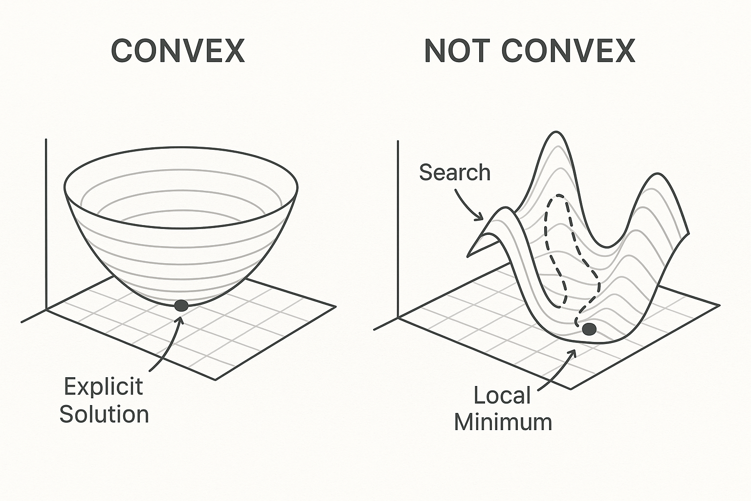
I first encountered a problem without a closed-form solution (outside of an academic setting) when I was building my Portfolio Optimizer program. In the simplest case of minimizing portfolio variance for a given return, the optimal weights can be solved for analytically. I used the Lagrange Multiplier method, which conceptually is just setting the gradient of the objective function to zero to find its minimum point. But, once you complicate the problem by, for example, introducing an inequality constraint such as disallowing short-selling (requiring weights ≥ 0%), the gradient becomes discontinuous and we can't express the weights explicitly anymore.
The way I think about it is that, for "nice" optimization problems (those with functions that are: convex, differentiable, and linear or quadratic), there are methods that allow you to do something similar to "solving for x". But, for more complex problems involving state-spaces that are more rugged, like those of non-convex functions, you must instead run an algorithm to iteratively search for the minimum. This process of iterative calculations is what we call a numerical method.
I. Polynomial/algebraic equations
Consider the simple linear equation $2x + 3 = 7$.
Nothing too surprising there. We were able to find a closed-solution by isolating $x$. But before investigating whether more complex equations have closed-solutions, how can we know whether a solution to a polynomial exists at all?
The Fundamental Theorem of Algebra states that every polynomial of degree n has exactly n complex roots.It's easy to visualize the FTA for functions with real roots (the three plots below). You can see that for a degree 1 polynomial (a line), there is always one root (where it crosses the x-axis), for degree 2 (a parabola) there are always two roots, and for degree 3 (a cubic curve) there are always three roots.
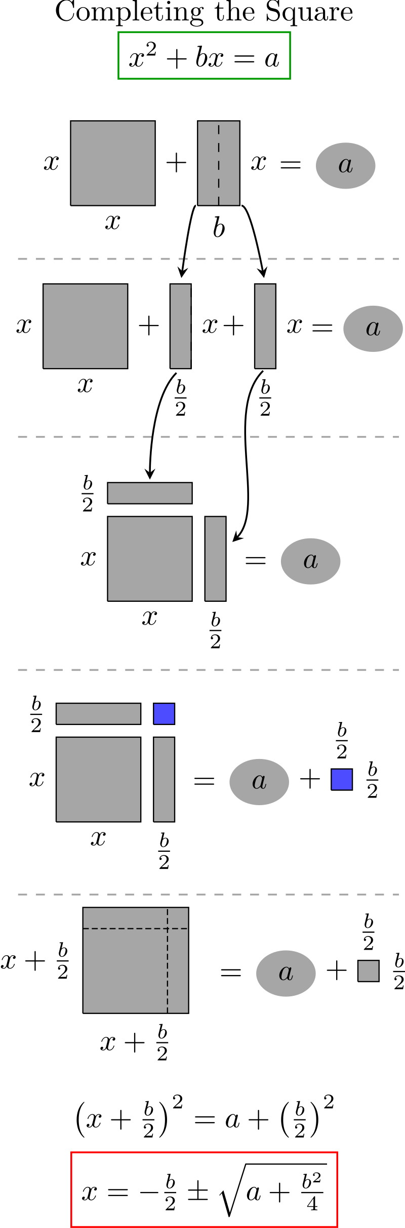
So, we know for certain that: (i) there exists exact solutions to all polynomials and (ii) some polynomials can be directly solved for using algebraic manipulation. It turns out that polynomials of degree 1-4 have closed-form solutions, and you can express them in a general formula. For example, quadratic equations (polynomials of degree 2) have a closed-form solution (the quadratic formula) that is taught in school. By ordering the equation into standard form $ax^2 + bx + c = 0$, we can directly apply the quadratic formula to find the roots.
By Krishnavedala - Own work, CC BY-SA 3.0, Link
This was discovered when some mathematicians, instead of rearranging terms of polynomials to solve for roots as we are used to, found ways to rearrange or "permute" the polynomial's roots themselves in a way that left the polynomial's coefficients unchanged. This might sound pretty abstract at first, but ultimately it is just a way of revealing the inherent structure of a polynomial by viewing it from different perspectives. To explain this further, we must introduce some additional terms and theory.
A symmetry of a system is a transformation that changes something about the system but leaves some other property unchanged, which we call an invariant. For example, rotating a perfect sphere changes its orientation but leaves its shape and size unchanged. A sphere has rotational symmetry that leave its shape invariant.Like a sphere, a polynomial can also have symmetries. The set of all symmetries that permute the polynomial's roots but leave the polynomial's coefficients unchanged is called its Galois group, $G$. Let's look at a simple example to see how this works in practice.
A solvable group is one whose symmetries can be broken down step-by-step until only the trivial symmetry (in this case, the identity) remains. Just a reminder, the identity symmetry can be represented as: $x \mapsto x$. Let's do a fully worked-out example using $f(x) = x^2 - 2$ again to see how this works.
II. Systems of linear equations
We began by looking at single polynomial equations, but what about systems of equations? Let's look at a system of two linear equations with two unknowns:
Well there are two requirements that guarantee a closed-form solution for linear systems. You can find other ways of stating these two requirements, but I find the most intuitive to be:
When to expect closed-form solutions for linear systems
- ✔System is determined: There are the same number of linear equations as unknown variables. In the above example there is one unknown, $x$, and one equation that contains that unknown.
- ✔System is linearly independent: One equation cannot be expressed as a linear combination of the others, meaning that the two equations encompass all the necessary information to find a unique solution in all of $\mathbb{R}^2$, or the coefficient vectors' "span" is equal to $\mathbb{R}^2$.
✔ It has two unknowns and two equations (it is determined)
✔ The equations are linearly independent, which you can show yourself by drawing their coefficient vectors $\mathbf{v_1} = \begin{pmatrix} 2 \\ 3 \end{pmatrix}$ and $\mathbf{v_2} = \begin{pmatrix} 4 \\ -1 \end{pmatrix}$ in 2D space and observing that they are not parallel.
II. Systems of non-linear equations
II. Numeric Solution Example
Now let's look at examples where there is no closed-form solution. Here is a very small numeric example that shows an iterative solver in action. We'll compute $\sqrt{2}$ by solving $x^2 = 2$ using Newton's method. This method produces a sequence of approximations $x_{n+1} = x_n - \frac{f(x_n)}{f'(x_n)}$ which converges rapidly for this problem.
Before going deeper, it helps to classify the kinds of problems we try to solve. One useful lens is that there are four common goal types in mathematics; this context makes it clearer when closed forms exist and when they usually do not.
Level I — Goal Type (What you’re trying to find)
| Category | Description | Typical Form | Closed-Form Chance |
|---|---|---|---|
| A. Equation / Root Finding | Find $x$ such that $f(x)=0$. | Polynomial, exponential, trigonometric equations. | High for linear or low-degree polynomials; falls rapidly for general nonlinear equations. |
| B. Optimization | Find $x$ minimizing or maximizing $f(x)$. | Linear, quadratic, or nonlinear objectives (with constraints). | Depends on convexity and constraints; closed form mostly for simple linear/quadratic with equality constraints. |
| C. Integration / Summation | Compute an area or total, $\int f(x)\,dx$ or $\sum f(x)$. | Integrals, series. | Often no closed form; numeric approximation (e.g., Simpson’s rule, Gaussian quadrature, Monte Carlo) is standard. |
| D. Differential / Dynamic Systems | Solve for a function $y(t)$ such that $F(y, y', t)=0$ (or systems/PDEs). | ODEs, PDEs, state-space models. | Rare closed forms; iterative or symbolic approximation dominates. |