Zero-Velocity Update Kalman Filter for ankle Position

Graduate Research — Boston University, 2020-2022

I implemented a Kalman filter to track ankle position during walking by integrating IMU acceleration. Integrating acceleration directly produces drift, so the filter uses zero-velocity updates (ZUPT) during stance phase to correct accumulated error. The measurement model simply checks if the predicted velocity is zero when the ankle contacts the ground.

📄 Published Paper

Koopman Pose Predictions for Temporally Consistent Human Walking Estimations

Conference paper describing the full pose estimation system incorporating ZUPT-based ankle tracking

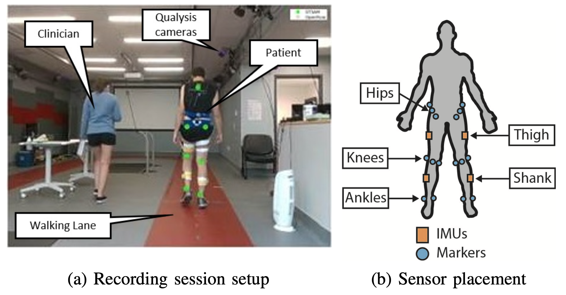
IMU sensor placement for ankle tracking during gait

Problem Setup

The state is position and velocity in one dimension:

$$\mathbf{x}_k = \begin{bmatrix} x_k \\ v_k \end{bmatrix}$$

During swing phase, only the predict step runs and uncertainty grows. During stance, the zero-velocity constraint corrects both velocity and position through the covariance structure.

Process Model

The state evolves according to standard equations of motion. Given previous state $\mathbf{x}_{k-1}$ and IMU acceleration $a_k$:

$$\hat{\mathbf{x}}_k^- = \mathbf{F}\hat{\mathbf{x}}_{k-1} + \mathbf{G}a_k$$

where

$$\mathbf{F} = \begin{bmatrix} 1 & \Delta t \\ 0 & 1 \end{bmatrix}, \quad \mathbf{G} = \begin{bmatrix} \frac{1}{2}\Delta t^2 \\ \Delta t \end{bmatrix}$$

The state transition matrix $\mathbf{F}$ propagates position and velocity forward in time. The input matrix $\mathbf{G}$ applies the measured acceleration to update the state.

Covariance Prediction

Uncertainty grows with each prediction:

$$\mathbf{P}_k^- = \mathbf{F}\mathbf{P}_{k-1}\mathbf{F}^T + \mathbf{Q}$$

$\mathbf{Q}$ is the process noise covariance representing IMU noise and model error. The term $\mathbf{F}\mathbf{P}_{k-1}\mathbf{F}^T$ propagates existing uncertainty through the linear transformation (analogous to $w\Sigma w^T$ in portfolio optimization).

Measurement Model

The measurement model extracts velocity from the state:

$$\mathbf{H} = \begin{bmatrix} 0 & 1 \end{bmatrix}$$

Multiplying the state by $\mathbf{H}$ gives the predicted velocity:

$$\hat{z}_k = \mathbf{H}\hat{\mathbf{x}}_k^- = v_k^-$$

During stance, the actual measurement is zero (ZUPT assumption: ankle velocity = 0). The residual is:

$$y_k = 0 - \hat{z}_k = -v_k^-$$

Kalman Gain and Update

The Kalman gain determines how much the state should move in response to the measurement residual:

$$\mathbf{K}_k = \mathbf{P}_k^- \mathbf{H}^T (\mathbf{H}\mathbf{P}_k^- \mathbf{H}^T + R)^{-1}$$

$R$ is the measurement noise covariance (a scalar for ZUPT, typically $R = 0.01$). The Kalman gain represents the covariance between the state and measurement, scaled by measurement uncertainty. It tells each state component how much to adjust when the residual is applied.

The state update applies the correction:

$$\hat{\mathbf{x}}_k = \hat{\mathbf{x}}_k^- + \mathbf{K}_k y_k$$

Here, $\mathbf{K}_k$ is a 2×1 vector (one entry for position, one for velocity). The Kalman gain is multiplied against the residual $y_k = -v_k^-$ to compute corrections for both position and velocity:

$$\begin{bmatrix} p_k \\ v_k \end{bmatrix} = \begin{bmatrix} p_k^- \\ v_k^- \end{bmatrix} + \begin{bmatrix} K_1 \\ K_2 \end{bmatrix} (-v_k^-)$$

This updates both states simultaneously: the velocity is directly corrected toward zero (via $K_2$), while the position is indirectly corrected (via $K_1$) thanks to the cross-covariance term in $\mathbf{P}_k^-$.

Covariance update:

$$\mathbf{P}_k = (\mathbf{I} - \mathbf{K}_k \mathbf{H})\mathbf{P}_k^-$$

How It Works

The filter alternates between two phases:

Swing phase: Only the predict step runs. Position and velocity are updated via equations of motion, and $\mathbf{P}_k$ grows as drift accumulates.
Stance phase: The zero-velocity update triggers. The residual $y_k = -v_k^-$ corrects both velocity directly and position indirectly through the cross-covariance in $\mathbf{P}_k$.

After many gait cycles, $\mathbf{P}_k$ converges to a repeating pattern reflecting typical uncertainty levels during each phase. The measurement noise $R$ determines how much to trust the ZUPT (low $R$ means strong trust). The process noise $\mathbf{Q}$ controls how quickly uncertainty grows during swing.

Uncertainty and Convergence

Why Covariance Converges

During each gait cycle, two competing processes act on the covariance matrix $\mathbf{P}_k$:

Predict step (swing): Uncertainty grows as $\mathbf{P}_k^- = \mathbf{F}\mathbf{P}_{k-1}\mathbf{F}^T + \mathbf{Q}$
Update step (stance): Uncertainty shrinks as $\mathbf{P}_k = (\mathbf{I} - \mathbf{K}_k\mathbf{H})\mathbf{P}_k^-$

After several gait cycles, these effects balance out and $\mathbf{P}_k$ converges to a steady pattern. The converged covariance tells you the typical accuracy of your position and velocity estimates.

Extracting Error Bounds

The covariance matrix $\mathbf{P}_k$ directly gives you uncertainty estimates:

$$\mathbf{P}_k = \begin{bmatrix} P_{11} & P_{12} \\ P_{12} & P_{22} \end{bmatrix}$$

The diagonal elements are variances. Take the square root to get standard deviations:

Position error: $\sigma_p = \sqrt{P_{11}}$ (e.g., 1.5 cm)
Velocity error: $\sigma_v = \sqrt{P_{22}}$ (e.g., 9 cm/s)

These standard deviations give you a ±1σ confidence interval (68% probability). For 95% confidence, use ±2σ.

Example After Convergence

Suppose after running the filter for a few steps, $\mathbf{P}_k$ settles to:

$$\mathbf{P}_k \approx \begin{bmatrix} 2.3 \times 10^{-4} & 1.1 \times 10^{-3} \\ 1.1 \times 10^{-3} & 8.7 \times 10^{-3} \end{bmatrix}$$

This means:

Position error: $\sigma_p = \sqrt{2.3 \times 10^{-4}} \approx 1.5$ cm
Velocity error: $\sigma_v = \sqrt{8.7 \times 10^{-3}} \approx 9.3$ cm/s
Off-diagonal $P_{12} > 0$ indicates position and velocity errors are correlated (when velocity estimate drifts high, position tends to overshoot)

Tuning for Better Accuracy

The converged uncertainty depends on your noise parameters:

Smaller $R$: Trust ZUPT measurements more → tighter convergence, smaller $\sigma_p$ and $\sigma_v$
Smaller $\mathbf{Q}$: Assume less IMU drift → slower uncertainty growth during swing

In practice, you run the filter for a few steps and check if $\mathbf{P}_k$ stabilizes. Once it does, you know your typical error margins.

Summary

The ZUPT Kalman filter corrects IMU integration drift by:

Predicting position and velocity using equations of motion during swing
Applying zero-velocity corrections during stance to reset accumulated error
Tracking uncertainty via the covariance matrix $\mathbf{P}_k$, which converges after a few steps

The standard deviations $\sigma_p = \sqrt{P_{11}}$ and $\sigma_v = \sqrt{P_{22}}$ give you practical error bounds on your estimates, typically around 1-2 cm for position and 5-10 cm/s for velocity with well-tuned parameters.